Visualization and analysis of legal texts
While browsing the Internet, you have probably seen a picture of a cloud filled with words of varying sizes that reflect the frequency of each word within a given text. This is referred to as a Tag Cloud or a Word Cloud. In this tutorial (see the notebook here), we will learn how to make Word Clouds in Python. This tool is useful for a visual exploration of text data.
We will use legal texts for the purpose of this tutorial, namely the Tunisian Constitution and the Tunisian Hydrocarbons Code.
As usual, we start by importing the different libraries used.
The NumPy library is used for handling large, multi-dimensional arrays and matrices.
For visualization, matplotlib is a comprehensive plotting library. It enables other libraries, such as seaborn and wordcloud, to run on its base.
The pillow library adds support for opening, manipulating, and saving many different image file formats.
from PIL import Image
from wordcloud import WordCloud, STOPWORDS
import pandas as pd
import numpy as np
import matplotlib.pyplot as plt
import re
import seaborn as sns
Generating Word Clouds
Then, we read the Hydrocarbons Code stored in a .txt file. I chose this legal document, because I have worked on it and analysed it for a thesis report I wrote. It is a complex legal text that pertains to a sensitive and important topic, that is natural resources.
We have to make some necessary text processing. First, we convert the entire text to lower case. This is important since Python strings are case sensitive. Afterwards, we use the magic of regular expressions to deal with apostrophes and other characters to be removed.
Whenever in doubt regarding regular expressions syntax, you can use this website or the official Python documentation to have the desired outcome.
hydrocarbons_code = open("hydrocarbons_code.txt", encoding='latin_1').read().replace("\n"," ")
hydrocarbons_code = hydrocarbons_code.lower()
hydrocarbons_code = re.sub(".'|[^\w ]", " ", hydrocarbons_code)
Since the text is in French, we have to make our own list (technically it’s a Python set with curly brackets here) of the words to remove from the given text. These words would not show in the Word Cloud.
If you do not speak French, most of these words are the equivalent to English articles, pronouns and conjunctions. They would not help us much in understanding the text through visuals.
stop = {'de','du','des','et','est','la','le','les','en','ou','par','au','aux','dans','une','un','pour','sur','ce','ces',
        'ne','qui','que','son','ses','sa','il','ci','a'}
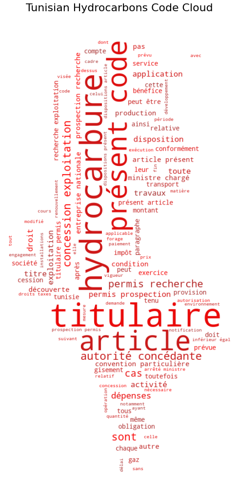
In order to create an image form for the Word Cloud, we need to use a PNG file as a mask. Here, I use the map of Tunisia, just for fun.
The mask argument in the WordCloud function takes an N dimensional array (ndarray). We use Image module to open the PNG file, and we transform it to the numpy array form.
According to WordCloud documentation, all white entries will be considerd masked out, while other entries will be free to draw on. In the NumPy array, all white parts of the mask have a value of 255, whereas values of 1 are black.
map_mask = np.array(Image.open("map.png"))
Now, we have a proper mask and we can make a cloud with the desired shape.
WordCloud takes several parameters, and you can create a personalised result by changing the optional arguments. Some of these are fairly self-explanatory. For the rest, you can always consult the relevant documentation. Or, you can check out the docstring of the function and see the required and optional arguments, by typing and running ?WordCloud.
hydrocarbons_cloud = WordCloud(max_words=1000, mask=map_mask, stopwords=stop , min_word_length = 3, min_font_size = 8,
                               margin=5, random_state=1, background_color="white", include_numbers=True).generate(hydrocarbons_code)
Finally, we can output the result and have an insightful and beautiful visualizations.
Naturally, the most frequent words are hydrocarbons, code, article and holder, as expected in a legal document about hydrocarbons!
%matplotlib inline
plt.figure(figsize=(18,18))
ax = plt.gca()
ax.set_title("Tunisian Hydrocarbons Code Cloud",fontsize=22)
plt.imshow(hydrocarbons_cloud.recolor(colormap=sns.color_palette(palette='blend:red,brown',as_cmap=True), random_state=3),
           interpolation="bilinear")
plt.axis("off")
plt.show()
#hydrocarbons_cloud.to_file("Hydrocarbons code cloud.png") #comment out to save the figure in a PNG format

Now, let’s take a look at the Tunisian Constitution. We will use an English translation from constitute project.
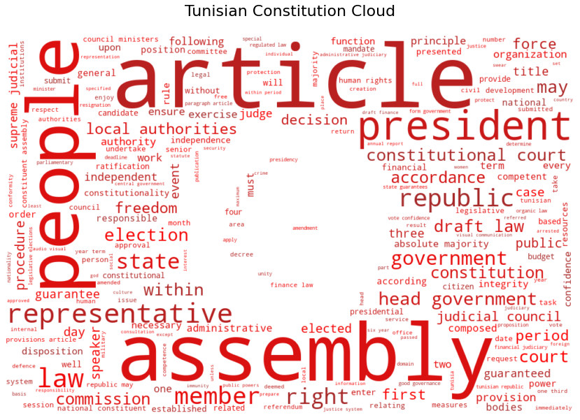
As before, we start by constructing a mask. For this example, it will be the Tunisian flag. For the rest, the only difference is that we use the default built-in STOPWORDS list.
flag_mask = np.array(Image.open("Flag_of_Tunisia.png"))

tunisian_constitution = open("constitution.txt").read().replace("\n"," ").lower()
tunisian_constitution = re.sub("[^\w ]", " ", tunisian_constitution)

constitution_cloud = WordCloud(max_words=1000, mask=flag_mask, stopwords=STOPWORDS , min_word_length = 3, min_font_size = 8,
                               margin=5, random_state=1, background_color="white", include_numbers=True).generate(tunisian_constitution)
Our exquisite result looks good, and presents us with useful visual anchor.
%matplotlib inline
plt.figure(figsize=(20,10))
ax = plt.gca()
ax.set_title("Tunisian Constitution Cloud",fontsize=22, y=1.04)
plt.imshow(constitution_cloud.recolor(colormap=sns.color_palette(palette='blend:red,brown',as_cmap=True)),
           interpolation="bilinear")
plt.axis("off")
plt.show()
#constitution_cloud.to_file("Tunisian Constitution Cloud.png") #comment out to save the figure in a PNG format

Counting words
However, text analysis goes beyond visualisations. We can count words using the Counter collection.
If we are only interested in the most common words, we can use .most_common() with or without an argument specifiying the number of words.
In the code below, we use list comprehension to store words appearing more than 30 times in the constitution and having at least 4 letters.
from collections import Counter
tunisian_words = [x for x in Counter(tunisian_constitution.split()).most_common(50) if x[1]>30 and len(x[0])>3 ]
tunisian_words
[('article', 173),
 ('shall', 173),
 ('assembly', 149),
 ('president', 110),
 ('people', 108),
 ('government', 100),
 ('representatives', 97),
 ('with', 97),
 ('republic', 96),
 ('state', 67),
 ('members', 62),
 ('court', 62),
 ('their', 50),
 ('draft', 48),
 ('head', 47),
 ('constitutional', 45),
 ('that', 43),
 ('laws', 42),
 ('within', 40),
 ('from', 39),
 ('right', 38),
 ('council', 37),
 ('judicial', 37),
 ('authorities', 34),
 ('local', 33),
 ('national', 32),
 ('after', 32),
 ('rights', 31),
 ('constitution', 31)]
Comparing different documents
We can compare the occurences of words in two documents as well. We will use the French constitution for comparison, despite the differences between the governance systems of the two countries as implemented in their respective constitutions.
We read and process the .txt file as we did before. Then, we store the words of each document in a list (tunisian_words and french_words).
french_constitution = open("french constitution.txt").read().replace("\n"," ").lower()
french_constitution = re.sub("[^\w ]", " ", french_constitution)

tunisian_words = tunisian_constitution.split(" ")
french_words = french_constitution.split(" ")
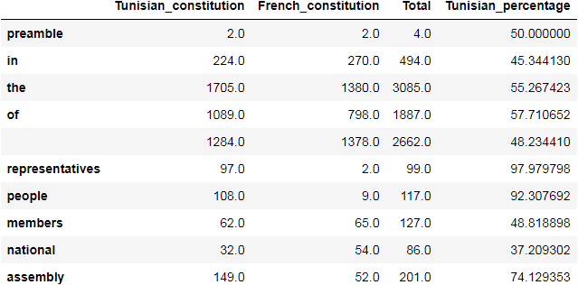
Afterwards, we construct a DataFrame by passing in the Counter collections as data entries, and setting the column labels.
In this example, we chose to remove missing values or drop them by using .dropna() with a 0 argument. That means, we drop rows which contain missing values. That would give us a DataFrame of only the words that exist in both documents!
The result below shows the number of occurrences of each word, the total, and a percentage value indicating the prevalence of that word in the Tunisian constitution with reference to its total use in both documents.
df = pd.DataFrame({
    'Tunisian_constitution': Counter(tunisian_words),
    'French_constitution': Counter(french_words)
}).dropna(0)

df['Total'] = df.Tunisian_constitution + df.French_constitution
df['Tunisian_percentage'] = (df.Tunisian_constitution / df.Total) * 100

df.head(10)

All of these common words between the two documents were used differently in each. We can check how many times they appeared by returning the sum of the values over the desired axis.
df.sum(axis = 0)
Tunisian_constitution    11950.000000
French_constitution      11769.000000
Total                    23719.000000
Tunisian_percentage      40472.171694
dtype: float64
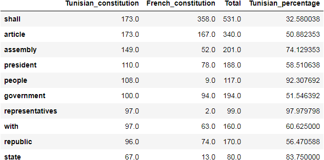
Now, let’s look at words used ten or more times in the Tunisian constitution. We sort them by descending value.
The for loop is used to go through df.index and remove the words having three characters or less.
for ind in df.index:
    if len(ind)<4:
        df.drop(ind, inplace = True)

df[df.Tunisian_constitution >= 10].sort_values(by='Tunisian_constitution', ascending=False)

We can use the df.sum() again to compute the frequency of those words.
df.sum(axis = 0)
Tunisian_constitution     5109.000000
French_constitution       5125.000000
Total                    10234.000000
Tunisian_percentage      34301.487972
dtype: float64
In this notebook (using python 3.7 pandas 1.2.1 and matplotlib 3.3.2), we have learned how to draw a Word Cloud that would be helpful for visualization of any text. Besides, we used Counter to count words in documents. The tool worked well with pandas DataFrames, allowing us to make simple comparisons.
This might have been naive text analysis, but it is an important first step towards a more comprehensive and elaborate text analysis.
Leave a comment